0%

NLP|谈谈预训练模型中的Adapter结构

最近应该会产出大量的关于预训练模型的解读的内容🤩,主要是目前预训练模型确实在几乎各个任务上的表现都超越了传统的模型。将预训练模型应用于各个领域,这也是一个大的趋势。这篇文章主要是通过AdapterBERT与K-Adapter两篇paper,来谈谈预训练模型中的Adapter结构。

Adapter-BERT

Adapter-Bert来源于Google的《Parameter-Efficient Transfer Learning for NLP》论文,主要目的在不降低模型效果的情况下,减小finetune时候的参数。感觉对于无GPU党来说,是一个非常大的福音。

背景

首先讲讲为什么要有Adapter-Bert。在预训练模型中,可以分为两种:feature-based以及fine-tuning。feature-based指的是通过预训练提取出词向量,然后输入到下游任务当中,在训练过程中,词向量可以随之更新,也可以不更新,侧重的是offline的词向量的生成,典型代表是ELM;fine-tuning指的是首先预训练模型,然后接入下游任务,将预训练阶段的权重作为finetuning的初始化权重,之后将下游任务与预训练部分一起训练,侧重的是co-training,典型代表是BERT。一般来说,fine-tuning的效果要比feature-based要好一些,当然计算代价也要更高一些。但是,总体而言,finetuning的代价实在是太大了,因为我们每一次都要更新所有的参数,这对很多应用尤其是低资源以及multi-mask的应用场景非常不友好。所以,我们想要尽可能地减少fine-tuning的所需要更新的参数数目,同时还要保证尽可能地逼近fine-tuning时的结果,于是便有了Adapter-BERT。

Adapter-BERT模型架构

Apdater-Bert的想法是将task-specific layer放在预训练模型中间,也就是加入Adapter结构,然后冻结住预训练模型参数,最后我们fientuning的时候,只更新Apdater、layerNorm以及与具体任务相关的layer的参数。具体结构图如下:

  • 左图是Adapter-BERT中的transformer layer,我们可以看到每一个transformer layer增加了两个Adapter layer,分别加在LayerNorm之前,当然了,在进行LayerNorm之前,我们需要进行讲Apdater layer的输出进行残差连接。
  • 右图是Adapter layer的具体结构示意。这个其实让我想到了ALBERT中的低秩因式分解。假设输入input的维度是$d$,我们首先通过一个FFN让其维度变为$m$,且$m<<d$;之后再通过一个FFN得到输出结果ouput,其其维度变为$d$。最后,我们进行残差连接,即input+output作为Adapter layer的输出结果。另外,分析一下Apdater layer的参数,对于一个transformer layer来说,增加的参数是2*(2dm+d+m+2d+2d),其中2d表示是LN的参数量,增加的参数量占总的参数量的3%。

思考一下,这里为什么要用残差连接?主要是因为当初始化的时候,权重都很小,残差连接可以保证模型输出与预训练模型相同。

实验结果

从结果来看,还是不错的,基本上能接近fine-tuning的结果。接下来看一下Ablation。

从结果中,我们可以得到如下结论:

  • 对于fine-tune来说,减小训练的层数会大幅降低准确率;而对于Adapter-based来说,几乎没有什么影响;
  • Fine-tune layerNorm没有什么用。

作者另外还做了很多实验,但是发现基本上没有什么影响。

代码部分

看完论文部分,我们来看一下代码实现部分。整体代码是在Google官方发布的BERT代码上改的,并且只修改了极小的一部分,首先是transformer部分,在每一个子层加上了Adapter layer。代码如下:

1
2
3
4
5
6
7
8
9
10
11
12
13
14
15
16
17
18
19
20
21
22
23
24
25
26
27
28
29
30
31
32
33
34
35
36
37
38
39
40
41
42
43
44
45
46
47
48
49
50
51
52
53
54
55
56
57
58
59
60
61
62
63
64
65
66
67
68
69
70
71
72
73
74
75
76
77
78
79
80
81
82
83
84
85
86
87
88
89
90
91
92
93
94
95
96
97
98
99
100
101
102
103
104
105
106
107
108
109
110
111
112
113
114
115
116
117
118
119
120
121
122
123
124
125
126
127
128
129
def transformer_model(input_tensor,
attention_mask=None,
hidden_size=768,
num_hidden_layers=12,
num_attention_heads=12,
intermediate_size=3072,
intermediate_act_fn=gelu,
hidden_dropout_prob=0.1,
attention_probs_dropout_prob=0.1,
initializer_range=0.02,
do_return_all_layers=False,
adapter_fn=None):
"""Multi-headed, multi-layer Transformer from "Attention is All You Need".

This is almost an exact implementation of the original Transformer encoder.

See the original paper:
https://arxiv.org/abs/1706.03762

Also see:
https://github.com/tensorflow/tensor2tensor/blob/master/tensor2tensor/models/transformer.py
Returns:
float Tensor of shape [batch_size, seq_length, hidden_size], the final
hidden layer of the Transformer.

Raises:
ValueError: A Tensor shape or parameter is invalid.
"""
if hidden_size % num_attention_heads != 0:
raise ValueError(
"The hidden size (%d) is not a multiple of the number of attention "
"heads (%d)" % (hidden_size, num_attention_heads))

attention_head_size = int(hidden_size / num_attention_heads)
input_shape = get_shape_list(input_tensor, expected_rank=3)
batch_size = input_shape[0]
seq_length = input_shape[1]
input_width = input_shape[2]

# The Transformer performs sum residuals on all layers so the input needs
# to be the same as the hidden size.
if input_width != hidden_size:
raise ValueError("The width of the input tensor (%d) != hidden size (%d)" %
(input_width, hidden_size))

# We keep the representation as a 2D tensor to avoid re-shaping it back and
# forth from a 3D tensor to a 2D tensor. Re-shapes are normally free on
# the GPU/CPU but may not be free on the TPU, so we want to minimize them to
# help the optimizer.

# [batch_size*seq_length,num_attention_heads*attention_head_size]
prev_output = reshape_to_matrix(input_tensor)

all_layer_outputs = []
for layer_idx in range(num_hidden_layers):
with tf.variable_scope("layer_%d" % layer_idx):
layer_input = prev_output

with tf.variable_scope("attention"):
attention_heads = []
with tf.variable_scope("self"):
attention_head = attention_layer(
from_tensor=layer_input,
to_tensor=layer_input,
attention_mask=attention_mask,
num_attention_heads=num_attention_heads,
size_per_head=attention_head_size,
attention_probs_dropout_prob=attention_probs_dropout_prob,
initializer_range=initializer_range,
do_return_2d_tensor=True,
batch_size=batch_size,
from_seq_length=seq_length,
to_seq_length=seq_length)
attention_heads.append(attention_head)

attention_output = None
if len(attention_heads) == 1:
attention_output = attention_heads[0]
else:
# In the case where we have other sequences, we just concatenate
# them to the self-attention head before the projection.
attention_output = tf.concat(attention_heads, axis=-1)

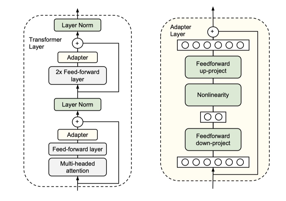
# Run a linear projection of `hidden_size` then add a residual
# with `layer_input`.
with tf.variable_scope("output"):
# [batch_size*seq_length,hidden_size]
attention_output = tf.layers.dense(
attention_output,
hidden_size,
kernel_initializer=create_initializer(initializer_range))
attention_output = dropout(attention_output, hidden_dropout_prob)
if adapter_fn:
# adapter结构
attention_output = adapter_fn(attention_output)
attention_output = layer_norm(attention_output + layer_input)

# The activation is only applied to the "intermediate" hidden layer.
with tf.variable_scope("intermediate"):
intermediate_output = tf.layers.dense(
attention_output,
intermediate_size,
activation=intermediate_act_fn,
kernel_initializer=create_initializer(initializer_range))

# Down-project back to `hidden_size` then add the residual.
with tf.variable_scope("output"):
layer_output = tf.layers.dense(
intermediate_output,
hidden_size,
kernel_initializer=create_initializer(initializer_range))
layer_output = dropout(layer_output, hidden_dropout_prob)
if adapter_fn:
# adapter 结构
layer_output = adapter_fn(layer_output)
layer_output = layer_norm(layer_output + attention_output)
prev_output = layer_output
all_layer_outputs.append(layer_output)

if do_return_all_layers:
final_outputs = []
for layer_output in all_layer_outputs:
final_output = reshape_from_matrix(layer_output, input_shape)
final_outputs.append(final_output)
return final_outputs
else:
# [batch_size,seq_length,hidden_size]
final_output = reshape_from_matrix(prev_output, input_shape)
return final_output

具体的Apdater layer代码如下:

1
2
3
4
5
6
7
8
9
10
11
12
13
14
15
16
17
18
19
20
21
22
23
24
25
26
27
28
29
30
31
32
33
34
35
36
37
38
39
40
41
42
43
44
45
46
47
def feedforward_adapter(input_tensor, hidden_size=64, init_scale=1e-3):
"""A feedforward adapter layer with a bottleneck.

Implements a bottleneck layer with a user-specified nonlinearity and an
identity residual connection. All variables created are added to the
"adapters" collection.

Args:
input_tensor: input Tensor of shape [batch size, hidden dimension]
hidden_size: dimension of the bottleneck layer.
init_scale: Scale of the initialization distribution used for weights.

Returns:
Tensor of the same shape as x.
"""
'''
input_tensor:[batch_size*seq_length,hidden_size]
'''
with tf.variable_scope("adapters"):
# in_size是self-attention layer的hidden_size,与这里的hidden_size不是一个概念!
in_size = input_tensor.get_shape().as_list()[1]
w1 = tf.get_variable(
"weights1", [in_size, hidden_size],
initializer=tf.truncated_normal_initializer(stddev=init_scale),
collections=["adapters", tf.GraphKeys.GLOBAL_VARIABLES])
b1 = tf.get_variable(
"biases1", [1, hidden_size],
initializer=tf.zeros_initializer(),
collections=["adapters", tf.GraphKeys.GLOBAL_VARIABLES])
# [batch_size*seq_length,hidden_size]
net = tf.tensordot(input_tensor, w1, [[1], [0]]) + b1

net = gelu(net)

w2 = tf.get_variable(
"weights2", [hidden_size, in_size],
initializer=tf.truncated_normal_initializer(stddev=init_scale),
collections=["adapters", tf.GraphKeys.GLOBAL_VARIABLES])
b2 = tf.get_variable(
"biases2", [1, in_size],
initializer=tf.zeros_initializer(),
collections=["adapters", tf.GraphKeys.GLOBAL_VARIABLES])
# [batch_size*seq_length,in_size]
net = tf.tensordot(net, w2, [[1], [0]]) + b2

# 残差连接
return net + input_tensor

这是模型部分,除此之外,修改的部分是:我们在fine-tune的时候,要冻结原来的预训练模型的参数,只更新新加的部分。这部分代码在optimization.py文件中,如下:

1
2
3
4
5
6
7
8
9
10
11
12
13
14
15
16
17
18
19
20
21
22
23
24
25
26
27
28
29
30
31
32
33
34
35
36
37
38
39
40
41
42
43
44
45
46
47
48
49
50
51
52
53
54
55
56
57
58
59
60
61
62
63
64
65
66
67
def create_optimizer(loss, init_lr, num_train_steps, num_warmup_steps, use_tpu):
"""Creates an optimizer training op."""
global_step = tf.train.get_or_create_global_step()

learning_rate = tf.constant(value=init_lr, shape=[], dtype=tf.float32)

# Implements linear decay of the learning rate.
learning_rate = tf.train.polynomial_decay(
learning_rate,
global_step,
num_train_steps,
end_learning_rate=0.0,
power=1.0,
cycle=False)

# Implements linear warmup. I.e., if global_step < num_warmup_steps, the
# learning rate will be `global_step/num_warmup_steps * init_lr`.
if num_warmup_steps:
global_steps_int = tf.cast(global_step, tf.int32)
warmup_steps_int = tf.constant(num_warmup_steps, dtype=tf.int32)

global_steps_float = tf.cast(global_steps_int, tf.float32)
warmup_steps_float = tf.cast(warmup_steps_int, tf.float32)

warmup_percent_done = global_steps_float / warmup_steps_float
warmup_learning_rate = init_lr * warmup_percent_done

is_warmup = tf.cast(global_steps_int < warmup_steps_int, tf.float32)
learning_rate = (
(1.0 - is_warmup) * learning_rate + is_warmup * warmup_learning_rate)

# It is recommended that you use this optimizer for fine tuning, since this
# is how the model was trained (note that the Adam m/v variables are NOT
# loaded from init_checkpoint.)
optimizer = AdamWeightDecayOptimizer(
learning_rate=learning_rate,
weight_decay_rate=0.01,
adapter_weight_decay_rate=0.01,
beta_1=0.9,
beta_2=0.999,
epsilon=1e-6,
exclude_from_weight_decay=["LayerNorm", "layer_norm", "bias"])

if use_tpu:
optimizer = tf.contrib.tpu.CrossShardOptimizer(optimizer)

#--------------------只更新后来新增的参数-------------------------------#

tvars = []
for collection in ["adapters", "layer_norm", "head"]:
tvars += tf.get_collection(collection)
grads = tf.gradients(loss, tvars)

# This is how the model was pre-trained.
(grads, _) = tf.clip_by_global_norm(grads, clip_norm=1.0)

train_op = optimizer.apply_gradients(
zip(grads, tvars), global_step=global_step)

#--------------------只更新后来新增的参数-------------------------------#

# Normally the global step update is done inside of `apply_gradients`.
# However, `AdamWeightDecayOptimizer` doesn't do this. But if you use
# a different optimizer, you should probably take this line out.
new_global_step = global_step + 1
train_op = tf.group(train_op, [global_step.assign(new_global_step)])
return train_op

到此,Adapter-BERT的论文预代码部分都讲完了☕️~
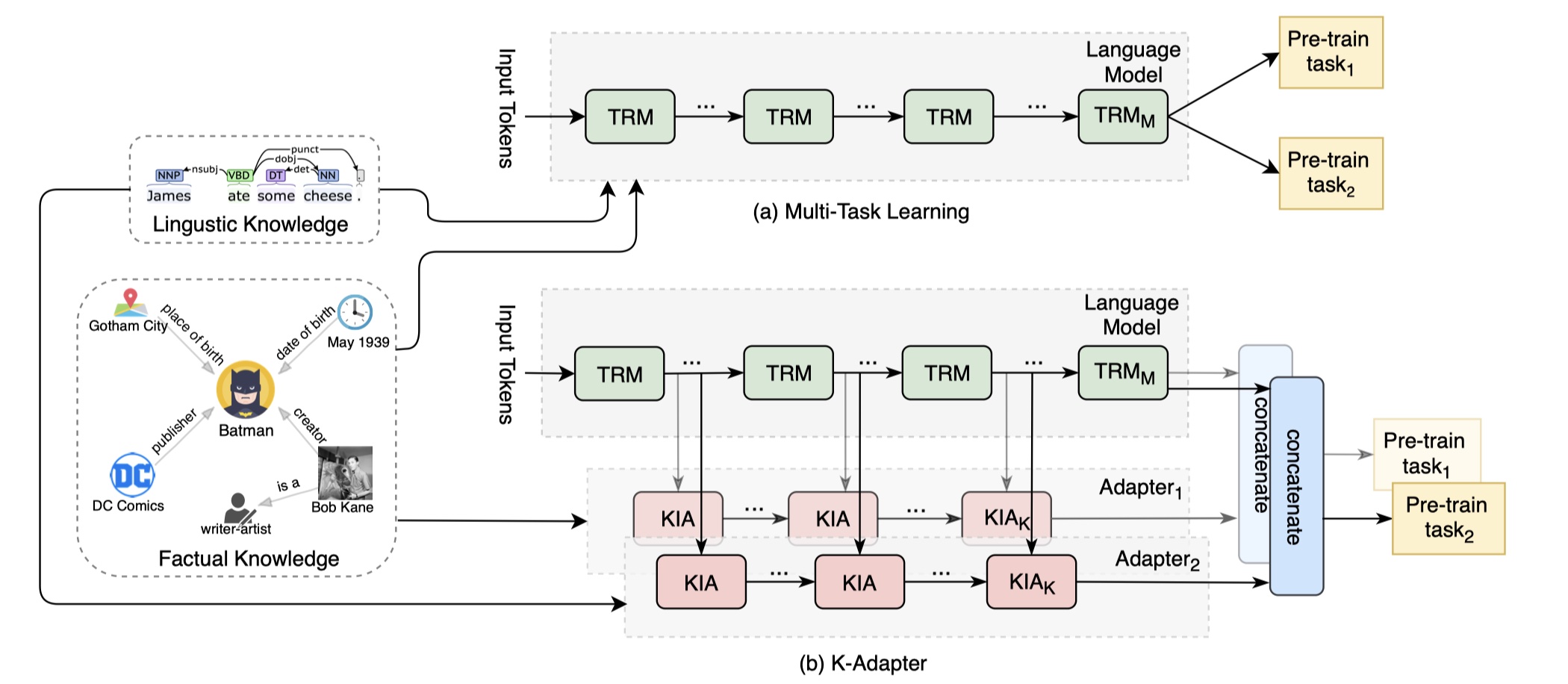
K-Adapter

K-Adapter模型来源于MSRA的《K-A DAPTER: Infusing Knowledge into Pre-Trained Models with Adapters》论文。它所要解决的问题是:在预训练模型中嵌入知识是非常重要的,因为当前的预训练模型无法学习到非常的知识信息;此外,在训练multi-task时,会出现灾难性遗忘问题,所谓的灾难性遗忘问题指的是:同一个模型,在学习完一个task之后,如果再学习新的任务,那么在原先的task上学习到的权重会被完全破坏掉,如果我们想要解决灾难性遗忘的问题,我们就需要用到持续学习。在这个背景下,K-Adapter预训练模型被提出来了。

K-Adapter模型架构

首先放一下K-Adapter预训练模型的架构图吧~

第一张图中的a部分表示的是传统的multi-task learning,b部分表示的是使用了K-Adapter结构之后的整体模型;第二张图表示的是Adapter layer。下面着重讲讲Adapter layer的构成以及模型是如何运作的。由于这篇paper没有放出源代码(都0202年,居然还有paper不放源代码🤷‍♂️),所以整体内容的理解只能从论文来获得。

  • 整篇paper是以RoBERTa预训练模型作为基准,来进行设计的;

  • 从整体来看,在使用了K-Adapter结构的模型中,我们是将Adapter结构独立出来,与pre-train model平行操作;此外,也不是每一个transformer layer都配有Adapter,在这篇paper里面, 是在RoBERTa Large 的第 0, 11, 23 层之后增加有 Adapter 层;

  • 对于每一种知识,我们都去设计一个对应的Adapter,即所有的Apdater都是knowledge-specific的,这样一来,每一种knowledge产生的representation都不会互相干扰,从而解决了多任务学习中的灾难性遗忘的问题;
  • 当我们只嵌入一种知识的时候,我们输出到task-specific layer的是knowledge-specific adapter最后一层的输出(最后一层的输出是pre-train model的输出与adapter的输出的concatenation);当我们嵌入多个知识的时候,我们输出到task-specific layer的是所有knowledge-specific adapters最后一层的输出的concatenation;
  • 对于单个 adapter layer,它的输入是:pre-train model中当前transformer层的输出结果与上一个adapter layer输出结果的concatenation;然后输入到一个投影层,即线性变换,然后再经过若干个transformer layer(论文是2个),然后使用残差连接,将最初的输入与经过多个transformer layer输出结果进行concatenation,作为这个adapter layer的输出结果;
  • 这篇paper使用了两种Adapter:factual Adapter与linguistic Adapter。factual Adapter 训练一个关系分类(relation classification)任务。通过判断三元组中 entity 是否存在相应关系来学习关系的知识。数据集是过滤 entity 出现小于 50 次的 T-RE-rc. 因为 Entity 长度不一,利用 Pooling 来对齐. 该任务训练 5epochs, Batch size 为 128;linguistic Adapter 则是完成预测依存关系中父节点 index 这个任务。数据集是利用 Stanford Parser 标注的 Book Corpus。因为是 token-level 的任务,最后过一个线性层输出到相应的分类。该任务训练 10epochs, Batch size 为 256;
  • 在预训练的时候,pre-trained model是frozen的,只训练Adapter结构;但是在fine-tune的时候,还是和BERT一样,pre-trained model、所有的Adapter结构以及task-specific layer一起进行参数的更新;
  • 与Adapter-BERT相比,K-Adapter更加侧重于对于多knowlwdge的处理以及灾难性遗忘的问题,而Adapter-BERT更加侧重于fine-tune阶段参数的减少。

实验结果

首先它对比了多个知识嵌入的预训练模型,我觉得还挺好的,如果之后在知识嵌入做文章的话,这里可以看作是一个小结~

然后我们来看一下实验结果~

上面三张图分别是在:细粒度实体类型预测任务、常识QA与开放域QA任务、关系分类任务上的结果,总的来说,采用Adapter结构的预训练模型的效果确实有所提升~

以上就是预训练Adapter结构的内容啦,之后可能会再关注一下知识嵌入的预训练模型吧,这是一个大的方向,感觉目前还是有搞头的,over☕️~

Would you like to buy me a cup of coffee☕️~